Virtual Datasets

Arraylake's native data model is based on Zarr Version 3. However, Arraylake can ingest a wide range of other array formats, including

• Zarr Version 2
• HDF5
• NetCDF3
• NetCDF4
• GRIB
• TIFF / GeoTIFF / COGs (Cloud-Optimized GeoTIFF)

Importantly, these files do not have to be copied in order to be used in Arraylake. If you have existing data in these formats already in the cloud, Arraylake can build an index on top of it. These are called virtual datasets. They look and feel like regular Arraylake groups and arrays, but the chunk data live in the original file, rather than in your chunkstore. Arraylake stores references to these files in the metastore.

caution

When using virtual datasets, Arraylake has no way to know if the files being referenced have been moved, changed, or deleted. Creating virtual datasets and then changing the referenced files can result in unexpected errors.

Working with Google Cloud Storage

While the examples below showcase datasets stored on Amazon S3, it is possible to use Virtual Datasets to reference datasets in Google Cloud Storage. To do so, set s3.endpoint_url:

from arraylake import Client, config

client = Client()
# set s3 endpoint for GCS + anonomous access
config.set({"s3.endpoint_url": "https://storage.googleapis.com"})
repo = client.get_or_create_repo("ORG_NAME/REPO_NAME")

NetCDF

In this example, we will create virtual datsaets from NetCDF files. The example file chosen is from Unidata's Example NetCDF Files Archive.

The specific file we will use is described as follows:

From the Community Climate System Model (CCSM), one time step of precipitation flux, air temperature, and eastward wind.

We have copied the file to S3 at the following URI: s3://earthmover-sample-data/netcdf/sresa1b_ncar_ccsm3-example.nc

First we connect to a repo

%xmode minimal

import xarray as xr
from arraylake import Client

client = Client()
repo = client.get_or_create_repo("earthmover/virtual-files")
repo

Output

Exception reporting mode: Minimal

Output

<arraylake.repo.Repo 'earthmover/virtual-files'>

Adding a file is as simple as one line of code. The second argument to add_virtual_netcdf tells Arraylake where to put the file within the repo hierarchy.

s3_url = "s3://earthmover-sample-data/netcdf/sresa1b_ncar_ccsm3-example.nc"
repo.add_virtual_netcdf(s3_url, "netcdf/sresa1b_ncar_ccsm3_example")

tip

The signature for all "virtual" methods mirrors cp source destination, so pass the remote URI first followed by the path in the repo where you want to ingest data.

We can see that several arrays have been added to our dataset from this one file.

print(repo.root_group.tree())

Output

/
 └── netcdf
     └── sresa1b_ncar_ccsm3_example
         ├── time (1,) >f8
         ├── ua (1, 17, 128, 256) >f4
         ├── lon_bnds (256, 2) >f8
         ├── pr (1, 128, 256) >f4
         ├── time_bnds (1, 2) >f8
         ├── lat (128,) >f4
         ├── msk_rgn (128, 256) >i4
         ├── lat_bnds (128, 2) >f8
         ├── lon (256,) >f4
         ├── tas (1, 128, 256) >f4
         ├── area (128, 256) >f4
         └── plev (17,) >f8

We can check the data to make sure it looks good. Let's open it with Xarray.

ds = xr.open_dataset(
    repo.store, group="netcdf/sresa1b_ncar_ccsm3_example", zarr_version=3, engine="zarr"
)
print(ds)

Output

/Users/deepak/miniforge3/envs/arraylake/lib/python3.11/site-packages/gribapi/__init__.py:23: UserWarning: ecCodes 2.31.0 or higher is recommended. You are running version 2.27.0
  warnings.warn(

Output

<xarray.Dataset> Size: 3MB
Dimensions:    (lat: 128, lon: 256, bnds: 2, plev: 17, time: 1)
Coordinates:
  * lat        (lat) float32 512B -88.93 -87.54 -86.14 ... 86.14 87.54 88.93
  * lon        (lon) float32 1kB 0.0 1.406 2.812 4.219 ... 355.8 357.2 358.6
  * plev       (plev) float64 136B 1e+05 9.25e+04 8.5e+04 ... 3e+03 2e+03 1e+03
  * time       (time) object 8B 2000-05-16 12:00:00
Dimensions without coordinates: bnds
Data variables:
    area       (lat, lon) float32 131kB ...
    lat_bnds   (lat, bnds) float64 2kB ...
    lon_bnds   (lon, bnds) float64 4kB ...
    msk_rgn    (lat, lon) int32 131kB ...
    pr         (time, lat, lon) float32 131kB ...
    tas        (time, lat, lon) float32 131kB ...
    time_bnds  (time, bnds) object 16B ...
    ua         (time, plev, lat, lon) float32 2MB ...
Attributes: (12/18)
    CVS_Id:              $Id$
    Conventions:         CF-1.0
    acknowledgment:       Any use of CCSM data should acknowledge the contrib...
    cmd_ln:              bds -x 256 -y 128 -m 23 -o /data/zender/data/dst_T85.nc
    comment:             This simulation was initiated from year 2000 of \n C...
    contact:             ccsm@ucar.edu
    ...                  ...
    project_id:          IPCC Fourth Assessment
    realization:         1
    references:          Collins, W.D., et al., 2005:\n The Community Climate...
    source:              CCSM3.0, version beta19 (2004): \natmosphere: CAM3.0...
    table_id:            Table A1
    title:               model output prepared for IPCC AR4

ds.pr.plot()

Output

<matplotlib.collections.QuadMesh at 0x292fd6910>

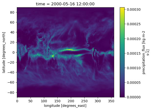
The data look good! All of the metadata made it through, and Xarray was able to use them to make a vert informative plot.

We're ready to commit.

repo.commit("Added virtual netCDF file")

Output

666a6a9e6eb92c4b69582861

Incrementally Overwrite Virtual Datasets

Now that our dataset is in Arraylake, we can incrementally overwrite it with new data. The new writes will be stored in our chunkstore; the original file will not be modified.

For example, imagine we discover that the precipitation field needs to be rescaled by a factor of 2:

pr_array = repo.root_group.netcdf.sresa1b_ncar_ccsm3_example.pr
pr_array[:] = 2 * pr_array[:]

We can see that only a single chunk of data was modified:

repo.status()

🧊 Using repo earthmover/virtual-files
📟 Session 21509b4f10c84e97aa5e2d2a96d100f5 started at 2024-06-13T03:42:22.436000
🌿 On branch main

paths modified in session

• 📝 data/root/netcdf/sresa1b_ncar_ccsm3_example/pr/c0/0/0

This new chunk has been stored the Arraylake chunkstore.

repo.commit("Rescaled precipitation")

Output

666a6aa0ad09014d212748ad

Other Formats

Zarr V2

If you have existing Zarr V2 data stored in object storage, you can ingest it virtually into Arraylake without making a copy of any of the chunk data.

As an example, we use a dataset from the AWS CMIP6 open data.

zarr_url = (
    "s3://cmip6-pds/CMIP6/CMIP/AS-RCEC/TaiESM1/1pctCO2/r1i1p1f1/Amon/hfls/gn/v20200225"
)

Let's first open it directly with xarray and see what's inside.

print(xr.open_dataset(zarr_url, engine="zarr"))

Output

<xarray.Dataset> Size: 398MB
Dimensions:    (time: 1800, lat: 192, lon: 288, bnds: 2)
Coordinates:
  * lat        (lat) float64 2kB -90.0 -89.06 -88.12 -87.17 ... 88.12 89.06 90.0
    lat_bnds   (lat, bnds) float64 3kB ...
  * lon        (lon) float64 2kB 0.0 1.25 2.5 3.75 ... 355.0 356.2 357.5 358.8
    lon_bnds   (lon, bnds) float64 5kB ...
  * time       (time) object 14kB 0001-01-16 12:00:00 ... 0150-12-16 12:00:00
    time_bnds  (time, bnds) object 29kB ...
Dimensions without coordinates: bnds
Data variables:
    hfls       (time, lat, lon) float32 398MB ...
Attributes: (12/53)
    Conventions:               CF-1.7 CMIP-6.2
    activity_id:               CMIP
    branch_method:             Hybrid-restart from year 0701-01-01 of piControl
    branch_time:               0.0
    branch_time_in_child:      0.0
    branch_time_in_parent:     182500.0
    ...                        ...
    title:                     TaiESM1 output prepared for CMIP6
    tracking_id:               hdl:21.14100/813dbc9a-249f-4cde-a56c-fea0a42a5eb5
    variable_id:               hfls
    variant_label:             r1i1p1f1
    netcdf_tracking_ids:       hdl:21.14100/813dbc9a-249f-4cde-a56c-fea0a42a5eb5
    version_id:                v20200225

Now let's ingest it into Arraylake.

repo.add_virtual_zarr(zarr_url, "zarr/cmip6_example")

ds = xr.open_dataset(
    repo.store, group="zarr/cmip6_example", engine="zarr", zarr_version=3
)
print(ds)

Output

<xarray.Dataset> Size: 398MB
Dimensions:    (time: 1800, lat: 192, lon: 288, bnds: 2)
Coordinates:
  * lat        (lat) float64 2kB -90.0 -89.06 -88.12 -87.17 ... 88.12 89.06 90.0
    lat_bnds   (lat, bnds) float64 3kB ...
  * lon        (lon) float64 2kB 0.0 1.25 2.5 3.75 ... 355.0 356.2 357.5 358.8
    lon_bnds   (lon, bnds) float64 5kB ...
  * time       (time) object 14kB 0001-01-16 12:00:00 ... 0150-12-16 12:00:00
    time_bnds  (time, bnds) object 29kB ...
Dimensions without coordinates: bnds
Data variables:
    hfls       (time, lat, lon) float32 398MB ...
Attributes: (12/51)
    Conventions:               CF-1.7 CMIP-6.2
    activity_id:               CMIP
    branch_method:             Hybrid-restart from year 0701-01-01 of piControl
    branch_time:               0.0
    branch_time_in_child:      0.0
    branch_time_in_parent:     182500.0
    ...                        ...
    table_id:                  Amon
    table_info:                Creation Date:(24 July 2019) MD5:0bb394a356ef9...
    title:                     TaiESM1 output prepared for CMIP6
    tracking_id:               hdl:21.14100/813dbc9a-249f-4cde-a56c-fea0a42a5eb5
    variable_id:               hfls
    variant_label:             r1i1p1f1

ds.hfls[-1].plot()

Output

<matplotlib.collections.QuadMesh at 0x2939e5210>

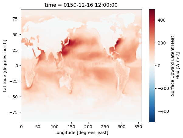
Data looks good! Let's commit.

repo.commit("Added virtual CMIP6 Zarr")

Output

666a6aa66eb92c4b69582862

GRIB

To demonstrate GRIB ingest, we'll use a GRIB file from the Global Ensemble Forecast System (GEFS)

grib_uri = "s3://earthmover-sample-data/grib/cape_sfc_2000010100_c00.grib2"
repo.add_virtual_grib(grib_uri, "gefs-cape/")
print(repo.to_xarray("gefs-cape/"))

Output

<xarray.Dataset> Size: 50MB
Dimensions:     (step: 24, latitude: 361, longitude: 720, number: 1,
                 surface: 1, time: 1, valid_time: 1)
Coordinates:
  * latitude    (latitude) float64 3kB 90.0 89.5 89.0 88.5 ... -89.0 -89.5 -90.0
  * longitude   (longitude) float64 6kB 0.0 0.5 1.0 1.5 ... 358.5 359.0 359.5
  * number      (number) int64 8B 0
  * step        (step) timedelta64[ns] 192B 10 days 06:00:00 ... 16 days 00:0...
  * surface     (surface) int64 8B 0
  * time        (time) datetime64[ns] 8B 2000-01-01
  * valid_time  (valid_time) datetime64[ns] 8B 2000-01-11T06:00:00
Data variables:
    cape        (step, latitude, longitude) float64 50MB ...
Attributes:
    centre:             kwbc
    centreDescription:  US National Weather Service - NCEP
    edition:            2
    subCentre:          2

We see a step dimension of size 24. Arraylake chooses to concatenate GRIB messages when it appears sensible to do so. However GRIB files comes in many varieties and can be hard to parse. Let us know if add_virtual_grib cannot ingest the GRIB file you want.

repo.commit("add gefs GRIB")

Output

666a6aab46079a62f6407336

Cloud-Optimized GeoTIFF

This section will demonstrate ingesting cloud-optimized GeoTIFFs (COG) virtually with Arraylake. It will discuss how Arraylake reads COGs virtually, which COGs are and aren't suitable for this method, as well as commonly encountered errors and how to resolve them.

A simple example

First, we will take a look at a straightforward example reading data from NASA's Ozone Monitoring Instrument (OMI) onboard the Aura satellite. The COG files are located in AWS S3 object storage, and information for accessing them can be found here.

no2_uri = "s3://omi-no2-nasa/OMI-Aura_L3-OMNO2d_2020m0531_v003-2020m0601t173110.tif"
repo.add_virtual_tiff(no2_uri, path="atmos_no2", name="2020_05_31")

Now that we've added the virtual file to our Repo's Zarr store, we can read the data with Xarray.

ds_no2 = xr.open_dataset(
    repo.store, group="atmos_no2/2020_05_31", engine="zarr"
)
print(ds_no2)

Output

/home/emmamarshall/miniconda/envs/arraylake/lib/python3.11/site-packages/gribapi/__init__.py:23: UserWarning: ecCodes 2.31.0 or higher is recommended. You are running version 2.27.0
  warnings.warn(

Output

<xarray.Dataset> Size: 5MB
Dimensions:  (Y: 720, X: 1440, Y1: 360, X1: 720, Y2: 180, X2: 360)
Dimensions without coordinates: Y, X, Y1, X1, Y2, X2
Data variables:
    0        (Y, X) float32 4MB ...
    1        (Y1, X1) float32 1MB ...
    2        (Y2, X2) float32 259kB ...
Attributes: (12/38)
    multiscales:              [{'datasets': [{'path': '0'}, {'path': '1'}, {'...
    Description:              Field=ColumnAmountNO2Trop,StdField=ColumnAmount...
    EndOrbit:                 18922
    EndUTC:                   2020-06-01T00:00:00.000000Z
    GranuleDay:               31
    GranuleDayOfYear:         152
    ...                       ...
    GeogCitationGeoKey:       WGS 84
    GeogAngularUnitsGeoKey:   9102
    GeogSemiMajorAxisGeoKey:  6378137.0
    GeogInvFlatteningGeoKey:  298.257223563
    ModelPixelScale:          [0.25, 0.25, 0.0]
    ModelTiepoint:            [0.0, 0.0, 0.0, -180.0, 90.0, 0.0]

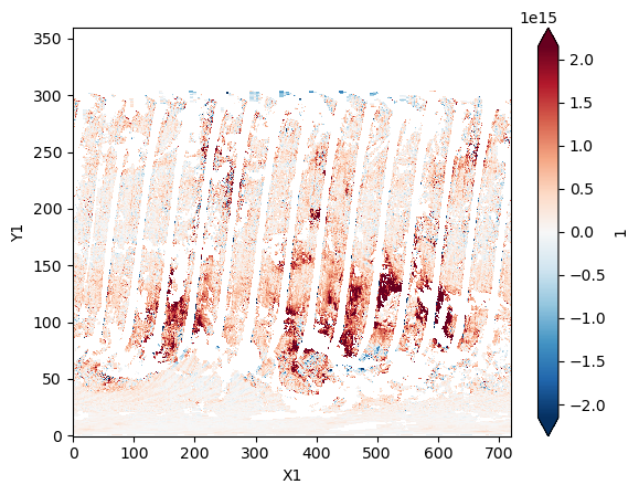
We successfully read an xr.Dataset that we ingested virtually from object storage. Taking a look at the dataset, we can see that there are three data variables that each exist along two dimensions, with six total dimensions in the xr.Dataset object. This is a COG with overviews, it provides views of the data at multiple spatial resolutions. Note that each 'overview' (data variable) is labelled with an integer, and the corresponding dimensions for that overview are suffixed with the same integer.

ds_no2["1"].plot(robust=True);

Commit the changes

repo.commit("added OMI virtual cog file")

Output

666a6abbad09014d21274925

GeoTIFFs encoded with non-standard codecs

Many TIFFs are encoded with codecs used for image compression and decompression. The imagecodecs library provides popular codecs such as LZW. Reading these TIFFs through Arraylake requires an extra step of registering the imagecodecs codec with numcodecs at read-time. If you encounter an error similar to 'ValueError: codec not available: 'imagecodecs_delta', you may need to import and register imagecodecs with numcodecs.

import imagecodecs.numcodecs

imagecodecs.numcodecs.register_codecs()

Now, we can virtually add a Sentinel-2 image COG. We are using a Sentinel-2 Level-2A product, which contains atmospherically corrected surface reflectance values. This is similar to the OMI example, but the Sentinel-2 object uses a different encoding system for chunk compression, which is why the prior step was necessary.

# mission = sentinel, sensor = s2, image date = 12/06/2023, processing level = l2a, band = b8a (narrow nir, 864-864.7 nm)
s2_uri = "s3://sentinel-cogs/sentinel-s2-l2a-cogs/54/H/YE/2023/12/S2A_54HYE_20231206_0_L2A/B8A.tif"
repo.add_virtual_tiff(s2_uri, path="sentinel-2", name="20231206")

Read the data with Xarray:

s2_ds = xr.open_dataset(repo.store, group="sentinel-2/20231206", engine="zarr")
print(s2_ds)

Output

<xarray.Dataset> Size: 161MB
Dimensions:  (Y: 5490, X: 5490, Y1: 2745, X1: 2745, Y2: 1373, X2: 1373,
              Y3: 687, X3: 687, Y4: 344, X4: 344)
Dimensions without coordinates: Y, X, Y1, X1, Y2, X2, Y3, X3, Y4, X4
Data variables:
    0        (Y, X) float32 121MB ...
    1        (Y1, X1) float32 30MB ...
    2        (Y2, X2) float32 8MB ...
    3        (Y3, X3) float32 2MB ...
    4        (Y4, X4) float32 473kB ...
Attributes: (12/14)
    multiscales:             [{'datasets': [{'path': '0'}, {'path': '1'}, {'p...
    OVR_RESAMPLING_ALG:      AVERAGE
    KeyDirectoryVersion:     1
    KeyRevision:             1
    KeyRevisionMinor:        0
    GTModelTypeGeoKey:       1
    ...                      ...
    GeogCitationGeoKey:      WGS 84
    GeogAngularUnitsGeoKey:  9102
    ProjectedCSTypeGeoKey:   32754
    ProjLinearUnitsGeoKey:   9001
    ModelPixelScale:         [20.0, 20.0, 0.0]
    ModelTiepoint:           [0.0, 0.0, 0.0, 699960.0, 6000040.0, 0.0]

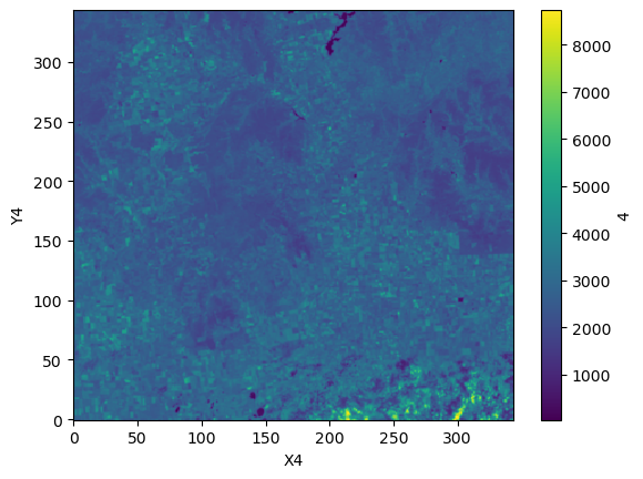
This xr.DataArray object is also an overview: it has 10 dimensions and 5 data variables; each data variable exists along two dimensions.

s2_ds["4"].plot();

repo.commit(message="Added s2 image")

Output

666a6abead09014d21274926

Considerations when virtually ingesting COGs

TIFF files are chunked internally, usually with very small chunk sizes (e.g. 256KB). Since Arraylake's add_virtual_tiff() method maps a single TIFF chunk to a single Zarr chunk, reading such virtual TIFFs with many small chunks may not be performant. For this reason, we arbitrarily limit virtual ingests to TIFF files with fewer than 500 chunks. Head here for an illustration of the internal chunking (tiling) of TIFF files.

The code below produces the error given by Arraylake when a dataset with too many chunks is added virtually.

capella_uri = "s3://capella-open-data/data/2021/3/10/CAPELLA_C02_SP_GEC_HH_20210310215642_20210310215708/CAPELLA_C02_SP_GEC_HH_20210310215642_20210310215708.tif"
repo.add_virtual_tiff(capella_uri, path="capella", name="Venice")

ValueError: The number of references > 500 is too large to ingest. This particular file is likely not a good fit for Arraylake. We recommend opening the file with rioxarray and writing it to Arraylakewith to_zarr.

The error tells us this dataset isn't a good candidate for adding virtually. Instead, we can read the data directly:

capella_ds = xr.open_dataset(capella_uri, engine="rasterio")
print(capella_ds)

Output

<xarray.Dataset> Size: 2GB
Dimensions:      (band: 1, x: 24489, y: 24529)
Coordinates:
  * band         (band) int64 8B 1
  * x            (x) float64 196kB 2.873e+05 2.873e+05 ... 2.959e+05 2.959e+05
  * y            (y) float64 196kB 5.039e+06 5.039e+06 ... 5.031e+06 5.031e+06
    spatial_ref  int64 8B ...
Data variables:
    band_data    (band, y, x) float32 2GB ...

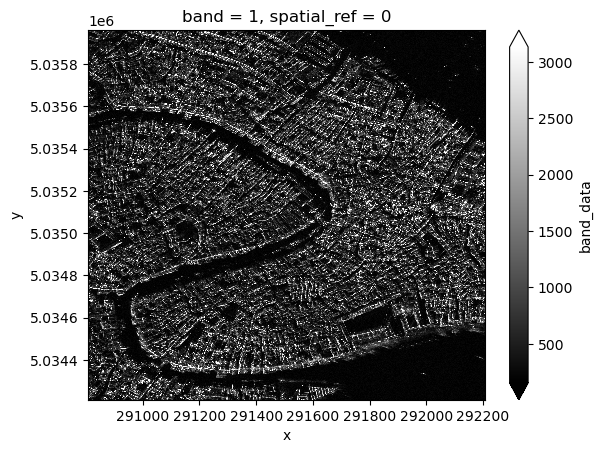
This object is pretty big. Subset it and write to Zarr

capella_sub = capella_ds.sel(band=1).isel(y=slice(10000, 15000), x=slice(10000, 14000))

capella_sub.band_data.plot(cmap="binary_r", robust=True);

capella_sub.to_zarr(repo.store, group="capella", mode="a");

repo.commit("Added capella data directly")

Output

666a6ae66eb92c4b69582933