Getting Started
Get started with Earthmover in 5 minutes by following this quick tutorial. This tutorial will explain:
- How to set up your account for the first time.
- How to subscribe to data on the Marketplace (ERA5).
- How to access your subscription ERA5 data using Xarray.
- How to access your subscription ERA5 data via compute services (map tiles and EDR).
- How to ingest your own private data.
The Earthmover Community Tier is free and full featured, including both storage and compute. See pricing for tier details.
Log in and create your org
The first time you sign up for Earthmover you will sign in and create a new organization (org). An org is necessary for this tutorial.
- Navigate to https://app.earthmover.io/auth/login and click "sign up".
- Enter your email address or use social login (Google, GitHub, or Microsoft)
- Once you're on the "Welcome to Arraylake" page, click on the violet "Create org" button.
- Pick a descriptive name for your organization. (Don't worry, the org is not publicly visible unless you explicitly make it so.) For example:
- Your company name
- Your research lab's name
- Your university department's name
- For individual personal use, consider using
{Your Name} Personal
- Click "I agree to the Terms of Service" (after reviewing the terms)
- Click the "Create" button to create your org.
After creating your org, you will be redirected to your org dashboard.
Remember your organization name. You will need it throughout this tutorial. We will refer to it as {ORG_NAME}.
Subscribe to Marketplace Data
The Data Marketplace offers over 60 PB of cloud-optimized, analysis-ready data at your fingertips. For this tutorial, we will use the free ERA5 Listing.
- From the org dashboard, click on "Browse marketplace"
- Search for ERA5 and scroll down to the free ERA5 listing, or navigate directly to https://app.earthmover.io/marketplace/6a19bcfe9aa6e97720a2fad2
- Click "Data Access"
- Click "Subscribe to this listing"
- In the dialog that pops up, keep the default name
era5-subscription - Click "Open Repo". This will bring you to your org's data catalog, where you can now view your subscription data.
Explore the Dataset
The Arraylake application allows you to browse and explore the dataset contents in the web.
Try clicking on single then spatial. Scroll down to view the data variables.
This ERA5 dataset has two distinct chunking schemes optimized for different types of queries:
Spatial subgroup ({group}/spatial/, valid_time=1, latitude=721, longitude=1440):
- One full global map per hour (pancake chunks)
- Optimized for map-style queries, regional extractions, spatial pattern analysis
- Fast access to complete spatial fields at specific times
Temporal subgroup ({group}/temporal/, valid_time=8736, latitude=12, longitude=12):
- One year of hourly data per chunk with small spatial tiles
- Optimized for time-series extraction, location-based analysis, ML training workflows
- Efficient loading of multi-year temporal sequences at fixed locations
We will use both in this tutorial.
Access data via Python and Xarray
Your subscription data can now be accessed anywhere on the internet where you can run Python. For this tutorial, use your local machine, a cloud-based notebook, or wherever you prefer to work!
First, you must install the Arraylake client and the Xarray library
pip install arraylake xarray
(Or use your preferred environment management tool like uv or conda.)
Then authenticate your client. From the shell, run:
arraylake auth login
Complete the authorization flow and then open a Python session (notebook, ipython, etc.).
To open your data with Xarray, run this code
from arraylake import Client
import xarray as xr

ORG_NAME = "my-org"  # your organization name goes here

client = Client()
repo = client.get_repo(f"{ORG_NAME}/era5-subscription")
session = repo.readonly_session(branch="main")
ds = xr.open_zarr(session.store, chunks=None, group="single/spatial")
print(ds)
You should see the same dataset you saw in the browser:
<xarray.Dataset> Size: 119TB
Dimensions:     (valid_time: 756048, latitude: 721, longitude: 1440)
Coordinates:
  * valid_time  (valid_time) datetime64[ns] 6MB 1940-01-01 ... 2026-03-31T23:...
  * latitude    (latitude) float64 6kB 90.0 89.75 89.5 ... -89.5 -89.75 -90.0
  * longitude   (longitude) float64 12kB 0.0 0.25 0.5 0.75 ... 359.2 359.5 359.8
    lsm         (latitude, longitude) float32 4MB ...
Data variables: (12/38)
    fdir        (valid_time, latitude, longitude) float32 3TB ...
    fsr         (valid_time, latitude, longitude) float32 3TB ...
    ie          (valid_time, latitude, longitude) float32 3TB ...
    hcc         (valid_time, latitude, longitude) float32 3TB ...
    d2m         (valid_time, latitude, longitude) float32 3TB ...
    fg10        (valid_time, latitude, longitude) float32 3TB ...
    ...          ...
    tp          (valid_time, latitude, longitude) float32 3TB ...
    u10         (valid_time, latitude, longitude) float32 3TB ...
    tcc         (valid_time, latitude, longitude) float32 3TB ...
    u100        (valid_time, latitude, longitude) float32 3TB ...
    v100        (valid_time, latitude, longitude) float32 3TB ...
    zust        (valid_time, latitude, longitude) float32 3TB ...
Attributes: (12/46)
    Conventions:                CF-1.7
    title:                      ERA5 Hourly Global Reanalysis - chunked for s...
    summary:                    ERA5 is the fifth generation ECMWF atmospheri...
    keywords:                   ERA5, reanalysis, atmosphere, climate, ECMWF,...
    keywords_vocabulary:        GCMD Science Keywords
    id:                         era5
    ...                         ...
    proj:code:                  EPSG:4326
    proj:epsg:                  4326
    GRIB_centre:                ecmf
    GRIB_centreDescription:     European Centre for Medium-Range Weather Fore...
    GRIB_subCentre:             0
    history:                    2026-07-07T11:48 GRIB to CDM+CF via cfgrib-0....
From here you can plot, analyze, and do anything you'd normally do in Xarray.
For example, to make a plot of a recent tcw value:
# Total column water vapor for a single hour, as a global map
ds["tcw"].sel(valid_time="2026-01-01T00:00").plot(figsize=(12, 5))
Or zoom into a specific region:
# Just over Europe
ds["tcw"].sel(
    valid_time="2026-01-01T00:00",
    latitude=slice(72, 34),
    longitude=slice(0, 40),
).plot()
This group is single/spatial, chunked so that each timestep is cheap to read
whole — ideal for maps. Pulling a long time series at one point would touch a
chunk per timestep instead. That is what the single/temporal group is chunked
for, and what the EDR service below is built to serve.
Access data via compute services
In addition to the direct access mode you saw above, Earthmover allows you to run compute and processing services on top of your data, which make it accessible for different applications and purposes.
Visualization: web map tiles
For geospatial data like ERA5, it's natural to want to view it on a map. Earthmover makes this easy with the Tiles service.
To activate Tiles from the web app:
- First make sure you're still on the dataset page:
https://app.earthmover.io/{ORG_NAME}/era5-subscription/tree/main/single/spatial - Click the button to switch from "Browse" to "Data Access"
- Click on "Web Map Tiles"
- Click "Deploy Map Tiles"
- Use all of the default settings and then click "add"
Your tiles service will start spinning up. This may take a few minutes.
Running compute services consumes compute credits. Don't worry, your service will automatically suspend itself after 15 minutes of inactivity. See Pricing for details.
Once tiles has started you'll be able to explore the data interactively.
Click on Variables and select tcw (total column water vapor).
An interactive map will appear, as shown below.
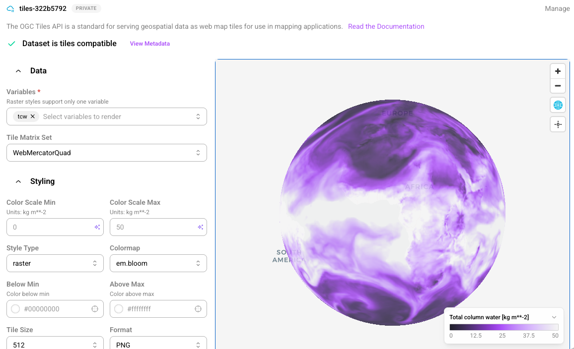
Choosing a variable on the left renders it live from the deployed Tiles service. The styling controls modify the look and feel of the generated tiles.
You can use your tile service outside of the Arraylake web app, in your own apps and dashboards! It works with any standard map tile application. See Tiles documentation for integration instructions.
Timeseries: EDR
Map tiles answer "what does this look like everywhere, right now". The other common question is the opposite one — "what does this look like here, over time". Environmental Data Retrieval (EDR) answers that over plain HTTP, returning a timeseries for a point without you downloading the dataset around it.
Deploy it the way you deployed Tiles, but from the single/temporal group,
which is chunked for reading through time:
- Go to
https://app.earthmover.io/{ORG_NAME}/era5-subscription/tree/main/single/temporal - Switch from "Browse" to "Data Access"
- Click "EDR", then "Deploy EDR", and accept the defaults
EDR endpoints are authenticated with your organization name as the username and
an Arraylake API token as the password. Create one under
https://app.earthmover.io/{ORG_NAME}/settings/api-clients.
Once the service is running, a position query returns CSV for one location:
curl -u {ORG_NAME}:{API_TOKEN} \
"https://compute.earthmover.io/v1/services/edr/{ORG_NAME}/era5-subscription/main/single/temporal/edr/position?coords=POINT(286.01%2040.75)&valid_time=2026-01-01T00:00:00/2026-01-07T23:00:00¶meter-name=t2m&f=csv"
Reading the query string:
coordsis a WKT point, longitude first, URL-encoded — the space becomes%20. The nearest grid cell is returned unless you addmethod=linear.- Longitudes must be given in the dataset's own convention. ERA5 runs from 0 to
360, so New York is
286.01, not-73.99. A longitude outside the grid is snapped to the nearest cell rather than rejected, which is a quiet way to get data for the wrong place — check thelongitudecolumn of the response. valid_timeis ERA5's time dimension. Any non-spatial dimension can be filtered by name this way, as a single instant or astart/endrange.parameter-namelimits the response to the variables you want, comma separated. Leave it off and you get all of them.f=csvsets the output format.geojson,nc, andparquetare also available, and the default is CoverageJSON.
The response is one row per timestep, ready to load straight into pandas:
import pandas as pd
df = pd.read_csv(
"https://compute.earthmover.io/v1/services/edr/{ORG_NAME}/era5-subscription"
"/main/single/temporal/edr/position"
"?coords=POINT(286.01%2040.75)"
"&valid_time=2026-01-01T00:00:00/2026-01-07T23:00:00"
"¶meter-name=t2m&f=csv",
storage_options={"auth": ("{ORG_NAME}", "{API_TOKEN}")},
)
See the EDR reference for area and cube queries, which return polygons and gridded subsets the same way.
Ingesting private data
Earthmover is not just for consuming data from the Marketplace! You can ingest, manage, and compute on your own private data.
Setting up a bucket
In order to ingest data, you need a storage bucket attached to your account. You can either bring your own storage bucket or use Earthmover-managed storage. (See Managing Storage for details.) For this tutorial, we will set up an Earthmover-managed bucket.
Here are the steps to set up an Earthmover-managed bucket:
- In the app sidebar, click
Data -> Buckets. - Click "New Bucket"
- Click "Create an Earthmover-Managed Bucket"
Your new bucket will now be accessible.
Create an empty Icechunk repo
Data is ingested to an Icechunk repo, managed by Arraylake. To create a new repo:
- In the web app sidebar, click
Data -> Repositories. - Click
New Repository -> Create Empty Repository - Name your repo
ingestion-test.
Ingest sample data via Xarray
You can ingest data from anywhere you can run Python.
First, connect to the repo you just created:
from arraylake import Client

client = Client()
repo = client.get_repo(f"{ORG_NAME}/ingestion-test")
Next, load some of Xarray's tutorial data:
import xarray as xr

air_temp = xr.tutorial.open_dataset(
    "air_temperature"
).chunk("1mb")
rasm = xr.tutorial.open_dataset(
    "rasm"
).chunk("1mb")
Then use Xarray to write to the repo:
# Start an icechunk session
session = repo.writable_session(branch="main")

# write the data to zarr
air_temp.to_zarr(
    session.store,
    group='air_temperature'
)
rasm.to_zarr(
    session.store,
    group='rasm'
)

# commit the data
session.commit("My first commit 🥹")
Now go back to the web app. You should see the data you just ingested. You can now access it, share it, and run compute services on top!