ECMWF Reanalysis 5 (ERA5) Surface
Data source
The source files are located at NSF NCAR Curated ECMWF Reanalysis 5 (ERA5).
ERA5 is the fifth-generation global reanalysis produced by the Copernicus Climate Change Service at ECMWF. It provides hourly estimates of atmospheric, land-surface and ocean variables from January 1940 to the present on a ~31 km (0.25°) grid, resolving 137 model levels up to 0.01 hPa; a 10-member 4D-Var ensemble supplies uncertainty information. The NSF NCAR Curated ERA5 collection republishes these data as CF-compliant NetCDF-4 files on AWS, delivering the hourly analyses and 12-h forecasts from both the high-resolution run and its ten-member ensemble on the same 0.25° grid—ready for large-scale research and ML/AI weather-model training.
The Arraylake / Icechunk edition is an analysis-ready dataset (ARD) that retains only the single-level surface fields—18 hourly variables such as 2 m temperature, 10 m wind, surface pressure, cloud cover, snow depth, and total-column water vapour—spanning 1975-01-01 to 2024-12-31. Rechunked into a ~60 TB Icechunk Zarr v3 store, it supports fast spatial and temporal slicing, making it ideal for climate research and for training ML/AI weather-forecast models.
Arraylake Repo
The ERA5-Surface Arraylake repo is named earthmover-public/era5-surface-aws and can be browsed at:
https://app.earthmover.io/earthmover-public/era5-surface-aws
Sub-groups
spatialchunks are (time=1,latitude=721,longitude=1440)—one full global map per hour—so map-style and regional queries load fast.temporalchunks are (time=8736,latitude=12,longitude=12)—equivalent to 1 year of hourly data and small chunksizes in latitude and longitude ideal for temporal queries and machine learning work flows.
Both groups contains 18 hourly single-level surface variables on the 0.25° grid (1975-01-01 → 2024-12-31).
Open Repo and explore contents
Let’s instantiate an Arraylake client, point it at the Earthmover API, and grab the earthmover-public/era5-surface-aws repo so we can open it with xarray.
from arraylake import Client

client = Client()  # call client.login() next if you haven't already
repo = client.get_repo("earthmover-public/era5-surface-aws")
Establish a read-only view of the immutable “main” branch
session = repo.readonly_session("main")
Open the spatial group with Xarray
import xarray as xr

ds_spatial = xr.open_dataset(
    session.store,
    engine="zarr",
    consolidated=False,
    zarr_format=3,
    chunks=None,
    group="spatial",
)
ds_spatial is now an xarray Dataset object that streams data on demand, ready for inspection or analysis.
print(ds_spatial)
<xarray.Dataset> Size: 33TB
Dimensions:    (time: 438312, latitude: 721, longitude: 1440)
Coordinates:
  * longitude  (longitude) float64 12kB 0.0 0.25 0.5 0.75 ... 359.2 359.5 359.8
  * latitude   (latitude) float64 6kB 90.0 89.75 89.5 ... -89.5 -89.75 -90.0
  * time       (time) datetime64[ns] 4MB 1975-01-01 ... 2024-12-31T23:00:00
Data variables: (12/18)
    blh        (time, latitude, longitude) float32 2TB ...
    sd         (time, latitude, longitude) float32 2TB ...
    d2         (time, latitude, longitude) float32 2TB ...
    skt        (time, latitude, longitude) float32 2TB ...
    cape       (time, latitude, longitude) float32 2TB ...
    stl1       (time, latitude, longitude) float32 2TB ...
    ...         ...
    tcc        (time, latitude, longitude) float32 2TB ...
    swvl1      (time, latitude, longitude) float32 2TB ...
    v100       (time, latitude, longitude) float32 2TB ...
    tcwv       (time, latitude, longitude) float32 2TB ...
    u10        (time, latitude, longitude) float32 2TB ...
    tcw        (time, latitude, longitude) float32 2TB ...
Attributes:
    DATA_SOURCE:  ECMWF: https://cds.climate.copernicus.eu, Copernicus Climat...
    Conventions:  CF-1.6
    history:      Created by Earthmover PBC on 2025-07-07 22:26:57 by combini...
Total dataset size in TB (terabytes)
size_tb = ds_spatial.nbytes / 1024**4
print(f"Dataset size: {size_tb:.1f} TB")
Dataset size: 29.8 TB
Spatial Query and Plot
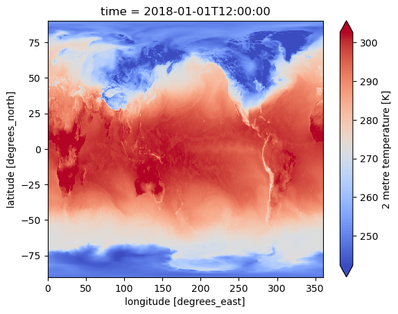
Extract a single-hour slice of 2 m air temperature and render it as a global map for 1 Jan 2018 12 UTC
ds_spatial.t2.sel(time="2018-01-01 12:00").plot(cmap="coolwarm", robust=True)
<matplotlib.collections.QuadMesh at 0x7329f7ffdb80>
Timseries Query and Plot
Similarly, we can open the temporal group by passing the parameter group="temporal" to xarray.open_dataset.
import xarray as xr

ds_temp = xr.open_dataset(
    session.store,
    engine="zarr",
    consolidated=False,
    zarr_format=3,
    chunks=None,
    group="temporal",
)
ds_temp is now an xarray Dataset object ready for temporal analysis.
print(ds_temp.data_vars)
Data variables:
    mslp     (time, latitude, longitude) float32 2TB ...
    sd       (time, latitude, longitude) float32 2TB ...
    cape     (time, latitude, longitude) float32 2TB ...
    sst      (time, latitude, longitude) float32 2TB ...
    d2       (time, latitude, longitude) float32 2TB ...
    sp       (time, latitude, longitude) float32 2TB ...
    tcwv     (time, latitude, longitude) float32 2TB ...
    swvl1    (time, latitude, longitude) float32 2TB ...
    skt      (time, latitude, longitude) float32 2TB ...
    t2       (time, latitude, longitude) float32 2TB ...
    stl1     (time, latitude, longitude) float32 2TB ...
    tcc      (time, latitude, longitude) float32 2TB ...
    tcw      (time, latitude, longitude) float32 2TB ...
    blh      (time, latitude, longitude) float32 2TB ...
    u10      (time, latitude, longitude) float32 2TB ...
    v100     (time, latitude, longitude) float32 2TB ...
    u100     (time, latitude, longitude) float32 2TB ...
    v10      (time, latitude, longitude) float32 2TB ...
The size of the ds_temporal is exactly the same as the data was rechunked for time-series analysis
size_tb = ds_temp.nbytes / 1024**4
print(f"Dataset size: {size_tb:.1f} TB")
Dataset size: 29.8 TB
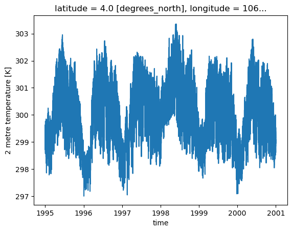
Extract multi-year slice of 2 m air temperature and render it as a time-series plot from 1995 to 2000 for a given location
ds_temp.t2.sel(longitude=106, latitude=4, time=slice("1995", "2000")).plot()
[<matplotlib.lines.Line2D at 0x7329f69a76e0>]
Both, spatial and temporal datasets contain:
- ➕ 18 hourly surface variables (e.g., skt, cape, u10, swvl1)
- 📐 Dimensions: time (438 312) × latitude (721) × longitude (1 440)
- 🌍 Coordinates: latitudes −90 → 90 °, longitudes 0 → 360 °
- 💾 Total size: ~30 TB stored in Zarr v3 / Icechunk format
- 📝 Global attributes and CF-1.6 metadata (data source, history, conventions)